A Primer on Automatic Differentiation#
This notebook explores the core capabilities of automatic differentiation (AD). The central idea of AD is to efficiently compute the action of the Jacobian matrix, rather than materializing the large matrix itself.
The Jacobian: The Full Derivative#
For any differentiable function \(f: \mathbb{R}^n \to \mathbb{R}^m\), its derivative at a point \(x\) is the unique linear map \(df_x: \mathbb{R}^n \to \mathbb{R}^m\) that provides the best linear approximation of the function’s change. The Jacobian matrix, \(J_f(x)\), is the matrix representation of this linear map with respect to the standard bases. It is an \(m \times n\) matrix of all first-order partial derivatives:
For complex models where \(n\) and \(m\) are large, constructing this matrix is often infeasible. AD provides an efficient way to compute its products with vectors.
1. Jacobian-Vector Product (JVP): The “Pushforward”#
The JVP is the core operation of forward-mode AD. It computes the directional derivative of the function \(f\) at a point \(x\) along a tangent vector \(v \in \mathbb{R}^n\). This is achieved by computing the product:
The result is a vector in the output space \(\mathbb{R}^m\) representing the rate of change of the output in the direction of \(v\). It gives a linear approximation of the function’s change: \(f(x+v) \approx f(x) + J_f(x)v\). This operation is computed without ever explicitly forming the full Jacobian matrix.
2. Vector-Jacobian Product (VJP): The “Pullback”#
The VJP is the core operation of reverse-mode AD, the engine behind backpropagation. It computes the product of the transposed Jacobian \(J_f(x)^T\) with a “cotangent” vector \(u \in \mathbb{R}^m\).
This operation “pulls back” the cotangent vector \(u\) from the output space to the input space. Its critical application is in the chain rule: if \(f\) is part of a larger composition \(g(x) = L(f(x))\), where \(L: \mathbb{R}^m \to \mathbb{R}\) is a scalar function, the VJP calculates the gradient of \(g\) when provided with the gradient of \(L\). Specifically, if \(u = \nabla L\), then \(\nabla g = \text{VJP}_f(x)(u)\).
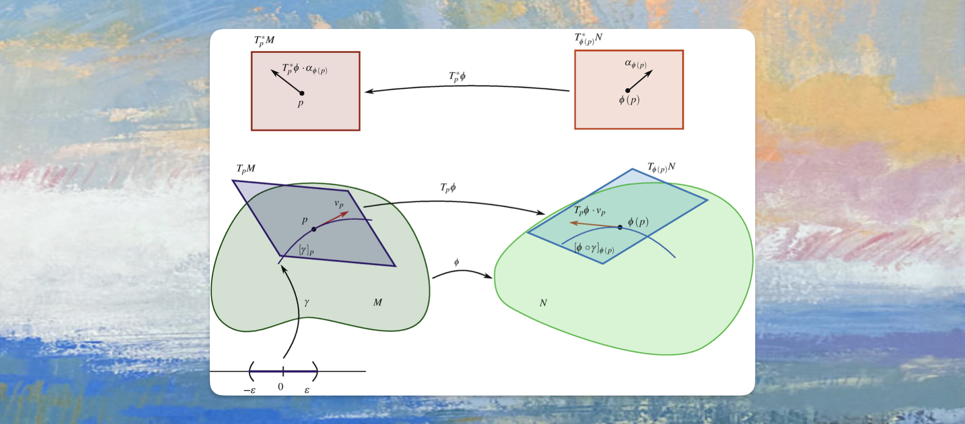
These terms and ideas have a rich meaning in the mathematical field of Differential Geometry, where they are often referred to as pushforward and pullback. The pushforward is the operation that takes a tangent vector from the input space and maps it to the output space, while the pullback takes a cotangent vector from the cotangent space and maps it back to the input’s cotangent space. Read more about that in this excellent Primer on Differential Geometry
In this notebook, we will use nabla to compute the JVP and VJP for a function \(f\) that takes an input from \(\mathbb{R}^{2k}\) and maps it to \(\mathbb{R}^k\), defined for inputs \((x_1, x_2)\) with \(x_1, x_2 \in \mathbb{R}^k\) as:
We will then see how these fundamental operations can be composed to construct the full Jacobian and second-order derivatives (the Hessian).
1. Setup#
[ ]:
import sys

try:
    import nabla as nb
except ImportError:
    import subprocess
    packages = ["nabla-ml"]
    subprocess.run([sys.executable, "-m", "pip", "install"] + packages, check=True)
    import nabla as nb

print(
    f"🎉 All libraries loaded successfully! Python {sys.version_info.major}.{sys.version_info.minor}"
)
2. Example Function Definition#
[ ]:
def my_program(x1: nb.Tensor, x2: nb.Tensor) -> nb.Tensor:
    a = x1 * x2
    b = nb.cos(a)
    c = nb.log(x2)
    y = b * c
    return y
3. Compute a regular forward pass.#
[2]:
# init input tensors
x1 = nb.tensor([1.0, 2.0, 3.0])
x2 = nb.tensor([2.0, 3.0, 4.0])
print("x1:", x1)
print("x2:", x2)

# compute the value of the program
value = my_program(x1, x2)
print("fwd_output:", value)
x1: [1. 2. 3.]:f32[3]:cpu(0)
x2: [2. 3. 4.]:f32[3]:cpu(0)
fwd_output: [-0.288451   1.0548549  1.16983  ]:f32[3]:cpu(0)
4. Compute a JVP (Jacobian-Vector Product)#
[3]:
# init input tangents
x1_tangent = nb.randn_like(x1)
x2_tangent = nb.randn_like(x2)
print("x1_tangent:", x1_tangent)
print("x2_tangent:", x2_tangent)

# compute the actual jvp
value, value_tangent = nb.jvp(my_program, (x1, x2), (x1_tangent, x2_tangent))
print("value:", value)
print("value_tangent:", value_tangent)
x1_tangent: [1.7640524 0.4001572 0.978738 ]:f32[3]:cpu(0)
x2_tangent: [1.7640524 0.4001572 0.978738 ]:f32[3]:cpu(0)
value: [-0.288451   1.0548549  1.16983  ]:f32[3]:cpu(0)
value_tangent: [-3.7025769   0.74225295  5.3027043 ]:f32[3]:cpu(0)
5. Compute a VJP (Vector-Jacobian Product)#
[4]:
# compute value and pullback function
value, pullback = nb.vjp(my_program, x1, x2)
print("value:", value)

# init output cotangent
value_cotangent = nb.randn_like(value)
print("value_cotangent:", value_cotangent)

# compute the actual vjp
x1_cotangent, x2_cotangent = pullback(value_cotangent)
print("x1_cotangent:", x1_cotangent)
print("x2_cotangent:", x2_cotangent)
value: [-0.288451   1.0548549  1.16983  ]:f32[3]:cpu(0)
value_cotangent: [1.7640524 0.4001572 0.978738 ]:f32[3]:cpu(0)
x1_cotangent: [-2.223683    0.36850792  2.9121294 ]:f32[3]:cpu(0)
x2_cotangent: [-1.478894    0.37374496  2.390575  ]:f32[3]:cpu(0)
6. Compute the full Jacobian#
6.1 Jacobian via vmap + vjp aka. batched reverse-mode AD#
[5]:
jac_fn = nb.jacrev(my_program)
jacobian = jac_fn(x1, x2)
print("jacobian:", jacobian)
jacobian: [[[-1.2605538   0.          0.        ]
 [-0.          0.92090786  0.        ]
 [-0.          0.          2.975392  ]]:f32[3,3]:cpu(0), [[-0.8383503   0.          0.        ]
 [-0.          0.93399537  0.        ]
 [-0.          0.          2.4425075 ]]:f32[3,3]:cpu(0)]
6.2 Jacobian via vmap + jvp aka. batched forward-mode AD#
[6]:
jac_fn = nb.jacfwd(my_program)
# jac_fn = nb.jit(jac_fn)
jacobian = jac_fn(x1, x2)
print("jacobian:", jacobian)

x1_p = nb.tensor([3.0, 2.0, 3.0])
x2_p = nb.tensor([4.0, 5.0, 6.0])
jacobian2 = jac_fn(x1_p, x2_p)
print("jacobian2:", jacobian2)
jacobian: [[[-1.2605538  -0.         -0.        ]
 [ 0.          0.92090786  0.        ]
 [ 0.          0.          2.975392  ]]:f32[3,3]:cpu(0), [[-0.8383503  -0.         -0.        ]
 [ 0.          0.93399537  0.        ]
 [ 0.          0.          2.4425075 ]]:f32[3,3]:cpu(0)]
jacobian2: [[[2.975392 0.       0.      ]
 [0.       4.377841 0.      ]
 [0.       0.       8.073531]]:f32[3,3]:cpu(0), [[2.4425075 0.        0.       ]
 [0.        1.583322  0.       ]
 [0.        0.        4.146818 ]]:f32[3,3]:cpu(0)]
7. Compute the full Hessian automatically#
7.1 Hessian via Forward-over-Reverse AD#
[7]:
jac_fn = nb.jacrev(my_program)
hessian_fn = nb.jacfwd(jac_fn)
hessian = hessian_fn(x1, x2)
print("hessian:", hessian)
hessian: [[[[[  1.153804  -0.        -0.      ]
  [  0.         0.         0.      ]
  [  0.         0.         0.      ]]

 [[ -0.        -0.        -0.      ]
  [  0.        -9.493694   0.      ]
  [  0.         0.         0.      ]]

 [[ -0.        -0.        -0.      ]
  [  0.         0.         0.      ]
  [  0.         0.       -18.71728 ]]]:f32[3,3,3]:cpu(0), [[[ -0.96267235   0.           0.        ]
  [  0.           0.           0.        ]
  [  0.           0.           0.        ]]

 [[  0.           0.           0.        ]
  [  0.          -5.7427444    0.        ]
  [  0.           0.           0.        ]]

 [[  0.           0.           0.        ]
  [  0.           0.           0.        ]
  [  0.           0.         -12.75754   ]]]:f32[3,3,3]:cpu(0)], [[[[ -0.96267235  -0.          -0.        ]
  [  0.           0.           0.        ]
  [  0.           0.           0.        ]]

 [[ -0.          -0.          -0.        ]
  [  0.          -5.742745     0.        ]
  [  0.           0.           0.        ]]

 [[ -0.          -0.          -0.        ]
  [  0.           0.           0.        ]
  [  0.           0.         -12.757539  ]]]:f32[3,3,3]:cpu(0), [[[-0.5168097  0.         0.       ]
  [ 0.         0.         0.       ]
  [ 0.         0.         0.       ]]

 [[ 0.         0.         0.       ]
  [ 0.        -3.953551   0.       ]
  [ 0.         0.         0.       ]]

 [[ 0.         0.         0.       ]
  [ 0.         0.         0.       ]
  [ 0.         0.        -9.776351 ]]]:f32[3,3,3]:cpu(0)]]
7.2 Hessian via Reverse-over-Forward AD#
[8]:
jac_fn = nb.jacfwd(my_program)
hessian_fn = nb.jacrev(jac_fn)
hessian = hessian_fn(x1, x2)
print("hessian:", hessian)
hessian: [[[[[  1.153804   0.         0.      ]
  [  0.         0.         0.      ]
  [  0.         0.         0.      ]]

 [[  0.         0.         0.      ]
  [  0.        -9.493694   0.      ]
  [  0.         0.         0.      ]]

 [[  0.         0.         0.      ]
  [  0.         0.         0.      ]
  [  0.         0.       -18.71728 ]]]:f32[3,3,3]:cpu(0), [[[ -0.9626724   0.          0.       ]
  [  0.          0.          0.       ]
  [  0.          0.          0.       ]]

 [[  0.          0.          0.       ]
  [  0.         -5.7427444   0.       ]
  [  0.          0.          0.       ]]

 [[  0.          0.          0.       ]
  [  0.          0.          0.       ]
  [  0.          0.        -12.757539 ]]]:f32[3,3,3]:cpu(0)], [[[[ -0.96267235   0.           0.        ]
  [  0.           0.           0.        ]
  [  0.           0.           0.        ]]

 [[  0.           0.           0.        ]
  [  0.          -5.742745     0.        ]
  [  0.           0.           0.        ]]

 [[  0.           0.           0.        ]
  [  0.           0.           0.        ]
  [  0.           0.         -12.757539  ]]]:f32[3,3,3]:cpu(0), [[[-0.5168097  0.         0.       ]
  [ 0.         0.         0.       ]
  [ 0.         0.         0.       ]]

 [[ 0.         0.         0.       ]
  [ 0.        -3.953551   0.       ]
  [ 0.         0.         0.       ]]

 [[ 0.         0.         0.       ]
  [ 0.         0.         0.       ]
  [ 0.         0.        -9.776351 ]]]:f32[3,3,3]:cpu(0)]]
9. Conclusion#
Automatic Differentiation is a powerful tool that automates the complex process of calculating derivatives. By seamlessly obtaining gradients from standard Python code, we can build sophisticated computational workflows. This capability is the engine behind many advanced fields, from physics simulations to the gradient-based optimization that powers modern machine learning.
To see these principles in action, explore our tutorials on training a simple MLP and a full Transformer Neural Network from scratch in Nabla.